
Deep Field stellar photometric timeseries
This page describes a set of photometric timeseries for 28108 point sources in the CFHTLS Deep Fields. The four CFHTLS Deep Fields have been observed regularly since early 2003, first as part of the CFHTLS, and subsequently as part of the standard star calibration at CFHT. The CFHTLS data are now all public and the standard star calibration images are public the night they are taken. With a 10 year baseline in time, The Deep Fields thus offer a rich data set for studying variable objects.
Method
In brief, the time series were generated as follows:
- Selection: A catalog of point sources was selected from the Deep fields.
- Aperture Photometry: For each source and for each image, seeing-matched aperture photometry was performed.
- Zero-point corrections: Small zero-point corrections were applied to the magnitudes on an image-by-image basis.
- Photometric errors: The photometric uncertainties (limited by flat fielding errors) were computed.
- Completeness: The completeness in each band was assesed.
- Distribution: Download the data.
Point source selection
The list of stars is generated from the "Best seeing" Deep field stacks. The stacks are described on the Deep Fields (best seeing) page, but in summary they are coadded images made from the Deep fields images with the best image quality. All the GRIZ stacks have 0.65" seeing, while the U band has 0.8" seeing. The G-band image was used as a reference. The stellar locus was identified on a plot of FWHM vs. magnitude, as shown below. FWHM here is actually determined from the half-light radius, measured in pixels and converted into FWHM in arcseconds, by multiplying by 0.32.
The figure below shows the stellar locus for one of the Deep fields. At the bright end, the upturn in FWHM shows the onset of staturation. At the faint end, the stellar locus merges with compact galaxies. The criteria for the stellar catalog were set to be 17.5>G>24 and FWHM=0.65 +/- 15% as shown by the red lines.
Aperture photmetry
Aperture photometry was done for each point source in each image of the 11765 images available for the CFHTLS Deep Fields. The objects position in RA and Dec was converted to an extension number and pixel (X,Y) position using the MegaPipe astrometric calibration. The objects position was further refined by fitting a Gaussian function with the appropriate FWHM the image. This re-centring typically produced a 0.1 pixel (or 0.02 arcsecond) shift in position.
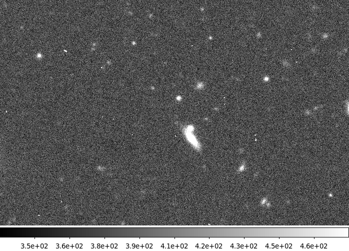
The sky was determined through an annulus with an inner radius of 70 pixels and an outer radius of 90 pixels. The figure below shows a bright star. The PSF has a bright core, and fainter, sharp-edged disk of light extending further. Depending on the star's location in the mosaic, this pupil image is generally not centred on the star. The 70 pixel inner radius insures that the disk of the pupil images does not lie in the annulus.
Next, aperture photometry was performed on each source through a series of apertures. There are a variety of photometric apertures that could be used: The CFHTLS Deep Fields were calibrated using SExtractor's MAG_AUTO which is a variable aperture Kron magnitude. It is optimized for galaxies, and is thus not necessarily approriate for stars. Fixed circle apertures are better, but the seeing in the CFHTLS image varies considerably, so a variable amount of light will be included in each aperture. If the aperture is large enough that the seeing effects won't matter, too much sky will be included and the random errors will be larger. To get around this, one must apply aperture corrections to correct to infinity. Finally one can use the seeing-matched aperture as adopted by Regnault et al. (2009). Here, the aperture is a fixed multiple of the IQ. This method has the benefit of allowing relatively small apertures that capture a consistent fraction of the light, obviating the need for aperture corrections. This is the method that was adopted. The question is: what multiple of the IQ should be used? Multiples from 1 to 9 times the seeing were tested. The zero-point/aperture corrections discussed below were applied. The photometric scatter of each object was measured. The objects were grouped by magnitude and the median scatter was determined.
The figure at right shows the photometric scatter as a function of magnitude, aperture and filter. For bright sources, the smallest scatter is generally found with an aperture 4 times the seeing. For fainter objects the scatter increases monotonically with aperture. To achieve the best possible photometry for the bright objects, an aperture of 4 times the seeing was adopted.
The aperture photometry was done using the CANFAR processing system. The IRAF aperture photometry package was used. The Deep fields are not crowded. PSF fitting photometry (e.g. DAOphot) does not provide any significant benefit.
Aperture/zero-point corrections
The photometric calibration of the CFHTLS Deep Fields was done using SExtractor's MAG_AUTO. MAG_AUTO is a Kron magnitude, primarily used for galaxy photometry. It builds an eliptical aperture based on the second order moments of the source. The more extended the source, the larger the aperture. The aperture ends up missing a small (2%) but consistent fraction of the light from a source, regardless of it's extent. This is obviously an advantage for galaxy photometry, but in general it is thought to be poor for stellar photometry, hence the use of aperture photometry for the project.
A correction is needed to convert between aperture photometry and MAG_AUTO. It turns out that if the aperture is a multiple of the IQ (rather than a fixed number of arcseconds) this correction has a pretty consistent value. The zero-point offset were measured for each of the 11765 Deep Field images. The aperture magnitudes measured in the images and the MAG_AUTO values from the stacks were compared. Only stars that appeared in all the images for a particular Deep field and filter were included in comparison. The zero-point/aperture correction was computed using artificial skepticism (Stetson 1989) to robustly reject any outliers due to cosmic ray hits or bad columns. The results are plotted below:
The figure below shows the zero-point difference between MAG_AUTO and mag(aper) as a function of aperture for the all the images, grouped by filter. When the aperture is only twice the IQ, the correction is on the order of +0.2 mags (MAG_AUTO collects more light than the aperture magnitude). At the large aperture end, the correction is -0.05 mags. Note that the curve of growth has not fully levelled off.
The grey curves represent indvidual images. The coloured dots and error bars show the average and RMS at each aperture. Most of the filters show two disctinct locii. The images in the lower locus were taken during two observing runs in 2007, when it seems the PSF profile was significantly different. There about 10-20 images in this locus out of the 2000 or some images in the main locus. Other this small number of exceptions, MAG_AUTO is an excellent proxy for an IQ-matched aperture.
The lower right panel shows the average corrections for all the filters together on the same plot.
The figure below shows the variation of the zero-point corrections as a function of IQ. It plots the difference between MAG_AUTO and magnitudes measured through an aperture 4 times the IQ, separated by filter. There are slight slopes, for each filter, but the difference between IQ=0.5" and IQ=1" ranges from 0.001 mags to 0.0045 mags, slightly less than the typical scatter of 0.005 mags. The new and the old I-filter are plotted together. This causes a slightly higher scatter on this plot. The distribution also appears slightly bimodal: the lower blob corresponds to the new I-filter. Again it appears that MAG_AUTO is an excellent proxy for an IQ-matched aperture over a range of seeing conditions.
These corrections were applied on a image-by-image basis. The corrections are available as ASCII file (DeepVarZPAP.gz).
Photometric errors
IRAF computes photometric uncertainties based on the read noise of the detector and Poission noise of the sky and the object. However it was discovered that, especially at the bright end, there was a considerably more scatter in the photometry than can be accounted for by Poisson noise alone.
This is illustrated by the figure below. The dots show the absolute difference between the magnitudes measured in a single image and the flux measured in the stacked image. The red line shows the median error as a function of magnitude The green line shows the median error as a function of magnitude reported by IRAF, which accounts for the read noise and Poission noise. At the bright end, the difference is about 0.01 magnitudes for this image. There are variations from image to image.
This discrepancy is important. One would like to measure the smallest possible variation in brightnesses, and not being able to measure magnitudes to better than 1%, even at bright magnitudes is unfortunate.
Other researchers have also failed to achieve better than 1% photometry with individual MegaCam images. Although the SNLS team achieves better than 1% photometry after combining several images together, and their zero-point calibration is better than 1%, comparing individual measurements of bright stars from image to image results in a scatter of typically 2% (Fabbro, private communication) Stetson (private communication) finds that a 1% error must be added in quadrature to the Possion uncertainties to account for the measured scatter.
After carefully investigating any possible errors in the zero-point determination and aperture corrections discussed above, the conclusion was reached that the errors may be occuring in the Elixir detrending stage. Images with a larger than usual descrepancy between Poisson and measured errors were examined by eye. These images showed visible problems either with fringes (in the Z-band) or flat-fielding. Examples are shown below.
The problem with this Z-band image is poor fringe subtraction.
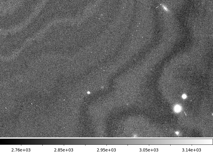
This image shows conspicuous background variations in the form of horizontal bands.
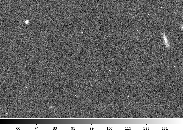
Here the problems are more subtle, but on careful examination, one can see patterns in the background. This is a G-band image; these are not fringes.
The conclusion is that although in most cases the the flat-fielding errors are too faint to be easily seen by eye, they nonetheless exist, and are responsible for the 0.01 mag floor in magnitude errors.
The magnitude errors reported in the distributed tables have been modified accordingly. The median measured errors are measured at 1 magnitude intervals for each image. This corresponds to the red line in the figure above. The errors given in the tables are linearally interpolated from these values. Below mag=22, the IRAF values are retained.
Completeness
Not every star is visible in every image. The images were taken with a dither pattern. Stars near the edge of a CCD in one image my lie completely outside the CCD in another image, either in the gap between the chips or completely outside the image area. Fainter stars may not be detected in an image taken in conditions of poor seeing, poor transparency, or increased sky brightness.
The figure below shows the recovery fraction as function of magnitude and filter. Recovery here means that the object was detected and that it's photometric uncertainty was better than 0.1 mags. Note that completeness is never 100%, because of the dithers.
Distribution
The time series are available as two tarballs each with 28108 files, one file per star. The files are in plain ASCII. The files have one row per image. When an object is not detected in a particular image, either because it was not located in a CCD or because it was too faint, the image is ommitted. Thus the files will not generally be the same length. There are two sets of files.
-
DeepVarTerse.tar.gz (625Mb):
These files give you only the following:
- Exposure midpoint (MJD)
- Magnitude
- Uncertainty in that magnitude
-
Number indcating the filter:
- 1: U
- 2: G
- 3: R
- 4: I
- 5: I2
- 6: Z
-
DeepVarFull.tar.gz (2.7Gb):
These files give you a bit more information. Each file has a
header which gives the UGRIZ magntitudes of the object in the
stack, as well as links to cutouts around each object in the
stacks. Each entry has a bit of extra information to allow one to
trace back any unsual object back to the object's position in a
particular image and ultimately back to the original photons.
- MegaCam exposure number
- Extension number in which object was detected
- X and Y in pixels in that image
- The image quality in arcseconds of the image
- Filter is given as a letter (UGRIZ and I2)
- A link to a cutout of around the object in the original object
- Date modified: